


The great ocean conveyor - what has it been doing lately?
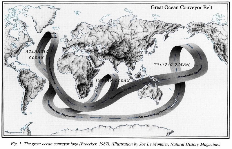
Figure 1. A schematic representation of the AMOC, from “The Great Ocean Conveyor” by Brocker (1991).
The great ocean conveyor belt is a colloquial term that is used to refer to the loosely organised band of currents that circulate around the world’s oceans. In the Atlantic sector, we’ve taken to calling this the ‘Atlantic meridional overturning circulation’ (aka AMOC) where near surface waters (top 1km) move northwards and deep currents (between 1km and 4km depth) move southwards. What is this system of currents? What has it been doing lately? Read on to find out more…
Oceans in Motion
In your bathtub, after you fill it, the water just kind of sits there peacefully, waiting for you to get in. Maybe there’s a bit of evaporation (steam) if it’s warm, but otherwise—just a large bucketful of water. The oceans are a different beast - rather than just sitting still (and maybe forming a few waves when the wind blows over the surface), there are currents and eddies all over the place. Currents are somewhat continuous patches of water that move together like a river, but without the riverbanks holding the water in on either side. The Gulf Stream is an example of one of these currents, which in this case runs northward along the east coast of the USA and then turns offshore around Cape Hatteras (35°N, 75°W) and extends across the North Atlantic.
The great ocean conveyor or Atlantic meridional overturning circulation is a ‘system of currents’—some northward flowing like the Gulf Stream, some southward flowing like the deep western boundary current (a southward flowing current between about 1-5km deep) and also found along the east coast of the USA (see Fig. 1). The reason we lump these currents together into a ‘system of currents’ is because together, they play an important role in the climate system. The northward flowing warm waters near the surface carry heat northward, while the deep southward currents are relatively colder, and they carry heat southward. The net effect of this circulation pattern is to bring heat from the south, release it to the atmosphere, and then return the now colder waters back to the south. We call this ‘overturning’ because when averaged over the whole Atlantic basin, the net effect is to tip the waters over—if there were a giant ferris wheel placed somewhere in the Atlantic (ok, you have to separate from reality a little here) then the northward flow near the surface would push the top half of the wheel northwards and the southward flow would push the bottom half southwards, and thus the wheel would rotate or ‘overturn’. See Fig. 2.
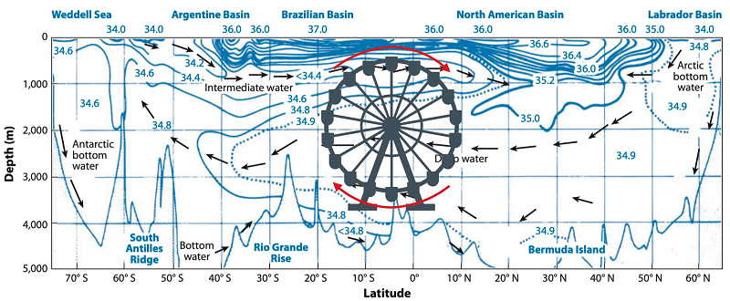
Figure 2. A meridional (north-south) section of salinity in the Atlantic, where the source waters at the equator could not have originated locally, and thus the overturning circulation (with source waters originating in the polar regions) was conjectured. From Lozier 2012. We added the ferris wheel with arrows of rotation to give the idea of how the northward flowing currents at 1000m, and the southward flowing currents at 2500m, lead to an ‘overturning’.
One of the reasons we’re interested in the AMOC is because of its role in moving heat around the climate system. Within the ocean, local warming causes sea level rise due to the expansion of water. When you move that heat somewhere else, you change the regional patterns of sea level rise. But if the warm water is at the surface—in contact with the atmosphere—it can also ‘release’ that heat to the atmosphere, basically warm the air above it which can cause storms (hurricanes are ‘fed’ by heat from the ocean) or change atmospheric circulation patterns (speeding up or slowing down the jet stream) and with it, weather.
How do we put a number on the strength of ocean circulation? “Sverdrups”
To quantify ocean heat, we talk about temperature—and it’s a matter of measuring the temperature of the water. For ocean currents, we need to know about velocity (speed and direction the water is moving). There are various ways to do this, but for a widespread current system like the AMOC we need to know about the ‘circulation’ which is an integration or ‘adding up’ of all the individual currents or velocity measurements in the top 1km and all the currents at depth, to see what the total overturning is. For ocean circulation, we talk about the strength of the circulation as a velocity times an area. Checking the units on this, velocity is measured in meters-per-second and area is meters-times-meters, so our circulation is measured in meters3/s (i.e. cubic meters per second), what we call a “transport” or a “volume transport”. For the AMOC, this means that when the number is larger, the ‘speed’ of the overturning is faster—and both the northward currents in the top 1km are faster *and* the southward currents below 1km are faster. On average, the strength of the AMOC is about 18,000,000 m3/s. That’s a lot of water. (By comparison, the Amazon River, one of the largest in the world, moves about 200,000 m3/s.) It’s also a lot of zeros, so we make our lives easier by defining a new unit, a ‘Sverdrup’ named after an oceanographer (Harald Sverdrup) where 1 Sverdrup or 1 Sv = 1,000,000 m3/s. By this measure, the average AMOC is about 18 Sv (and the Amazon River merely 0.2 Sv).
So then, what has the AMOC been doing lately?
(Note: ‘Lately’ for moored AMOC observations can mean a delay of 1 or more years.)
The latest measurements of the AMOC come from the RAPID 26°N array of moorings, which are scientific instruments installed or `deployed’ along the latitude 26°N in the Atlantic—roughly between Florida and the Canary Islands off of Morocco. These moorings are recovered approximately every 18 months to 2 years, at which point a research ship goes out to their location, pulls them up onto the ship and then scientists download the data from the instruments. After a multi-month process of checking the data quality and calibrations, then running the data through a series of computer codes, the strength of the AMOC can be estimated.
The latest expedition to service the RAPID moorings was in March 2022 for moorings near the Canary Islands, and December 2020 - January 2021 for moorings near the Bahamas. Both datasets are needed to produce the transports, so the AMOC strength is available updated to December 2020.
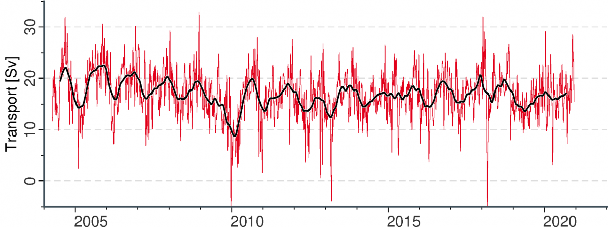
Figure 3. Strength of the AMOC at 26°N from the RAPID array (April 2004 - December 2020), where the red lines are at a nominal 10-day resolution, and the black line is the low-pass filtered variability.
This update from the RAPID array (Fig. 3) shows that the AMOC over the past year is about average. The average over the full record (2 April 2004 - 11 Dec 2020) is 16.9 Sv. Over 2020 (up until 11 Dec), the average strength of the MOC was 17.0 Sv. So - this is a bit anticlimatic. All that explanation and the effort to make the measurements - but this is unexpected.
A recent paper by Moat et al. (2020) actually predicted or at least hinted, that the AMOC was going to recover to its previous strength. (The average strength from April 2004 - April 2009 period was 18.5 Sv.) This was based on the evidence from the subpolar North Atlantic (the region north of about 40°N) that there was intense cooling and therefore a stronger ‘sinking’ limb of the AMOC around 2015 (Washington post: Cold Blob). Estimates of the overturning strength at 45°N based on atmospheric forcing that generated the cold blob suggested that the AMOC should increase, where these increases then move southward so that some time (ranging from a couple years to one decade) later, the increases would be seen at lower latitudes like 26°N. Instead, it looks like the AMOC strength has remained low (Fig. 4).
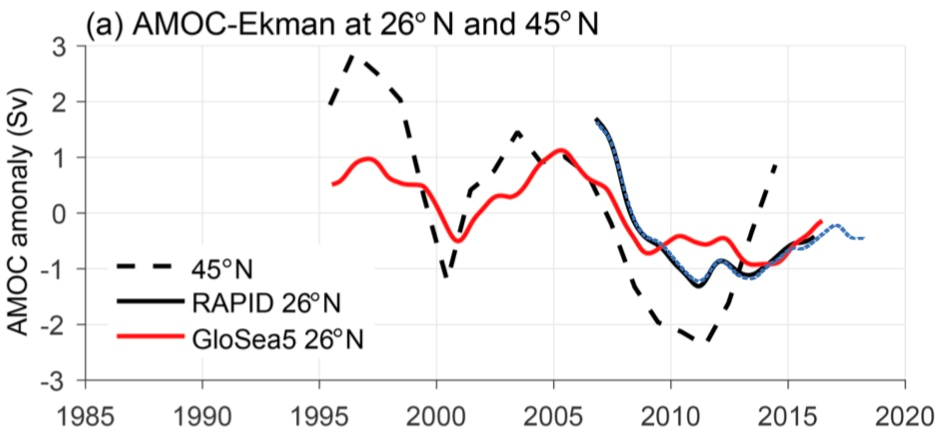
Figure 4. AMOC transport anomalies from 26°N, a model reanalysis and an estimate for 45°N based on the expected AMOC response to atmospheric forcing (from Moat et al. 2020). At the time the Moat et al. paper was written, RAPID data were available through 2018. The update through Dec 2020 is shown overlaid in the blue dashed line.
So, what's going on here?
On longer timescales, the cold blob is an expected consequence of an AMOC slowdown (Caesar et al. 2018), i.e. when the AMOC slows down, it transports less heat northward to the North Atlantic. In the particular case of the cold blob of 2015, the blob resulted largely from air-sea fluxes (Duchez et al. 2016). These same air-sea fluxes (intense cooling and watermass transformation) should intensify the AMOC - at least in the subpolar North Atlantic. If the AMOC behaves like a conveyor belt - even a conveyor belt with time lags, then the overturning strength further south (e.g. in the subtropical North Atlantic) should then also strengthen in response to the strong atmospheric forcing.
Was the cold blob unusual in other ways, maybe related to the ‘great salinity anomaly’ of 2014 when a flood of fresher-than-usual water entered the North Atlantic (Holiday et al. 2020).
Have we just not waited long enough to see the uptick in AMOC strength? (Watch this space–in February 2023, the RAPID 26°N moorings near Florida and the Bahamas are due to be serviced again, allowing an update of the 26°N time series through March 2022.)
What else are we missing?
Time will tell…
(Blog written by Dr. Eleanor Frajka-Williams)


Add new comment