


Recommendations from CLIVAR basin panels - Indian
The CLIVAR basin panels have been asked to provide WGOMD with input on ocean metrics to evaluate model performance in terms of ocean processes occurring in the different ocean basins. Return to main REOS Metrics page.
 |
 |
 |
 |
Metrics for the Indian Ocean
Recommendations from the CLIVAR Indian Ocean Panel
- Indian Ocean Indices
- Indian Ocean circulation and climate variability - Review paper by Schott et al. (2009)
- References
Indian Ocean Indices
The Indian Ocean Panel proposes six categories of indices to evaluate different aspects of the Indian Ocean region:
- Indian Ocean Dipole
- Indonesian Throughflow
- Arabian Sea
- Seychelles/Chagos Thermocline Ridge
- Leeuwin Current
- Western boundary currents
The names indicate relevant Indian Ocean Panel members.
Focus on Indian Ocean Dipole
Analysts: Tony Lee and Mike McPhaden (Tong.Lee@jpl.nasa.gov, Michael.J.Mcphaden@noaa.gov)
Time series at least though December 2006 are recommended to capture the large 2006 Indian Ocean Dipole (IOD) event and to facilitate comparison with moored ADCP time series observations.
a) Monthly SST in the IOD index regions
i) 50°E - 70°E, 10°S - 10°N
ii) 90°E - 110°E, 10°S - 0°
Anomalies of these two time series will define variability associated with the IOD.
b) Monthly sea level (in meters) in the same two regions as in (a). These give a measure of the time varying upper ocean mass distribution associated with IOD variability. Anomalies of these two indices can be readily validated against satellite altimetry beginning in 1992.
c) Surface wind stress (in N/m2)
i) Zonal wind stress averaged 2.5N-2.5S, 70-100E. This quantity is the principal dynamical forcing for IOD variability.
ii) Zonal and meridional wind stress averaged in the eastern IOD index region 90°E - 110°E, 10°S - 0° to provide a measure of local wind forcing.
d) Zonal volume transport integrated 2.5N-2.5S in the upper 200 m along 80E (in Sv). This quantity should be related to zonal wind stress forcing, zonal sea level differences and SST differences across the basin. The latitudinal range should capture most of the variability associated with the bienniel Wyrtki Jets. An ADCP transport array between 2.5N and 2.5S along 80E, to deployed in August 2009 for 3 years, could be used validation for this index in the future.
e) Zonal transport per unit width (i.e. depth integrated zonal velocity) at 0°, 80°E over the upper 200 m (in Sv/m). This quantity should be reasonably well correlated with zonal transport along 80°E and is more readily verified using moored velocity measurements from 1993-94 and 2004-present.
Indonesian Throughflow
Analysts: Susan Wijffels and Gary Meyers (Susan.Wijffels@csiro.au, Gary.Meyers@imos.org.au)
On time scales longer than about a year, transport across XBT line IX1 is a measure of Indonesian Throughflow from the Pacific. Monthly transport (0-800m) through IX1 (geostrophic plus Ekman, in Sv) should be calculated perpendicular to the XBT line.The end points of IX1 are Indonesian shelf (Sunda Strait) (approx. 6.5S, 105E) and Australian Shelf (off Shark Bay) (approx 25.5S 113E). Time series for 1983 to 2006 exist for comparison with ocean analyses.
Arabian Sea
Analysts: Gabe Vecchi and Jerry Wiggert (Gabriel.A.Vecchi@noaa.gov, jerry.wiggert@usm.edu)
a) SST in the regions 50E-60E, 5N-10N. This shows a strong correlation with Western Ghats rainfall.
b) Wind stress in the same region to compute offshore Ekman transport as an index for coastal upwelling.
c) SST in the region 16-19N, 57-62E as an index for biological studies.
Seychelles/Chagos Thermocline Ridge
Analyst: Jerome Vialard (vialardj@nio.org)
a) SST, sea level and mixed layer depth averaged over 5°S-10°S in two regions:
i) 60°E-80°E
ii) 80°E-100°E
b) Zonal transport (in Sv) in the upper 500m across 80°E between 5°S-10°S.
Leeuwin Current flow
Analysts: Ming Feng and Chari Patiaratchi (Ming.Feng@csiro.au, chari.pattiaratchi@uwa.edu.au)
The Leeuwin Current (LC) flows adjacent to the West and South coasts of Australia. Latitudinal changes occur in the strength of the LC three transects should be monitored:
a) Meridional transport across 24°S and 32S between 11°0E-coast in the upper 300m.
b) Zonal transport across the south coast at 118°E - from the coast to 38°S in the upper 300m.
c) It would also be valuable to look at Fremantle sea level at 32°S, 115E°
Western boundary currents
Analysts: Will De Ruijter (w.p.m.deruijter@phys.uu.nl) and Ridderinkhof and Van Leeuwen
a) The Mozambique Channel currents and transports across the narrowest section between Africa and Madagascar around 17 S; u,v, T,S-fields from top to bottom (for volume, overturning, T & S transports). This can be connected to the LOCO mooring array across the channel that has been in place near 17S since 2003 and will stay there at least for several more years.
b) Same for the East Madagascar Current at 24°S perpendicular to Madagascar coastline out to ± 400km. Analysis by Ridderinkhof, Van Leeuwen & De Ruijter. A mooring array has been proposed to NWO, the Dutch NSF.
c) Agulhas Current transports: u,v,T & S fields top to bottom perpendicular to the S. African coast near East London (33.4°S) along the Jason-1 groundtrack out to 30°E, 37°S. Analysis by Beal and others. A mooring array has been proposed to NSF.
d) Agulhas Leakage Index: this would need u,v fields top to bottom around South Africa, roughly between 0° and 50°E, 20° and 45°S. Feasibility depends on the possibility to connect numerical drifters to the model output. Analysis by Van Sebille, Van Leeuwen & De Ruijter.
Indian Ocean circulation and climate variability - Review paper by Schott et al. (2009)
"In recent years, the Indian Ocean (IO) has been discovered to have a much larger impact on climate variability than previously thought. This paper reviews climate phenomena and processes in which the IO is, or appears to be, actively involved. We begin with an update of the IO mean circulation and monsoon system. It is followed by reviews of ocean/atmosphere phenomenon at intraseasonal, interannual, and longer time scales. Much of our review addresses the two important types of interannual variability in the IO, El Niño–Southern Oscillation (ENSO) and the recently identified Indian Ocean Dipole (IOD). IOD events are often triggered by ENSO but can also occur independently, subject to eastern tropical preconditioning. Over the past decades, IO sea surface temperatures and heat content have been increasing, and model studies suggest significant roles of decadal trends in both the Walker circulation and the Southern Annular Mode. Prediction of IO climate variability is still at the experimental stage, with varied success. Essential requirements for better predictions are improved models and enhanced observations."
The following are some indices presented in the Schott et al. (2009) review on the Indian Ocean. Classification is based on time scales of interest: averaged fields, interannual and decadal variability, and linear trends. Refer to the paper online for full size figures.
Averaged Fields
--Depth of 20ºC isotherm (often referred to as Z20).
--The state of Z20 is reflected to the tropical SST and thus its reproducibility may affect amplitudes of climate variability such as ENSO and IOD, e.g., Figure 14 of Schott et al. (2009) as adopted from Xie et al. (2002).
Figure 14, Schott et al. (2009): Annual mean depth of the 20°C isotherm (contours in m) and correlation of its interannual anomalies with local SST (color shades) [from Xie et al., 2002].
--Comparison with WOCE sections: I8 (95ºE): Antarctic Intermediate Water, Subantarctic Mode Water, I3/I4 (20ºS): Mozombique Channel transport.
Interannual variability
--The first principal component of SST and Z20: a proxy for IO dipole, e.g., Figure 18a of Schott et al. (2009) as adopted from Saji et al. (2006).
Figure 18(a), Schott et al. (2009): IOD pattern during September–November. (a) Regression of 20°C isotherm depth (Z20; shades in m) and surface wind velocity (m/s) upon the first principal component of Z20 [from Saji et al., 2006a].
Decadal variability
--Variability of mixed layer depth of eastern IO (10ºS-0º, 90º-110ºE), e.g., Figure 28 of Schott et al. (2009) as adopted from Annamalai et al. (2005).
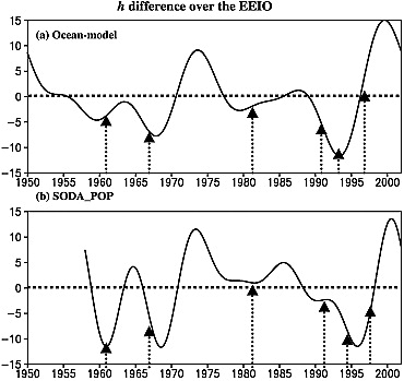
Figure 28, Schott et al. (2009): Mixed layer depth in eastern IO (10°S–0°; 90–110°E) in (a) ocean GCM driven by NCEP winds and (b) SODA assimilation model output. Vertical lines mark IOD occurrences [from Annamalai et al., 2005b].
Trends
--Linear trend of upper layer heat content (upper 700m) of Indian and Southern Indian Ocean, e.g., Figure 25a, b of Schott et al. (2009) as adopted from Levitus et al. (2000).
--Linear trend of zonally averaged temperature for the whole basin, e.g., Figure 25c-e of Schott et al. (2009) as adopted from Alory et al. (2007).
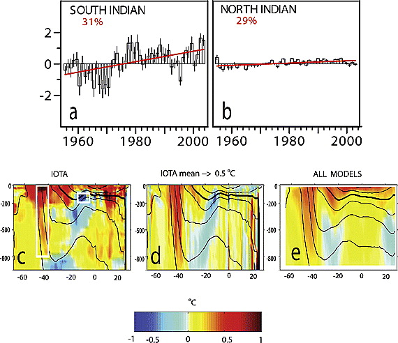
Figure 25, Schott et al. (2009): Time series 1955–2003 of yearly heat content (1022 J) of upper 700 m for (a) the southern and (b) the northern Indian Ocean, with vertical bars for ±1 standard deviation of the annual means. Red lines are the respective trends, and percentages are the variances explained by each trend line (reprinted from Science [Levitus et al., 2000]). (c) Zonally averaged temperature trends 1960–1999 (color shades) from new IO temperature archive (IOTA [from Alory et al., 2007]). (d) As Figure 25c but calculated after shifting mean temperature structure by 0.5° southward. (e) Trends from mean structure of 10 Intergovernmental Panel on Climate Change models.